Introduction to CASE for multi-cell-type eQTL fine-mapping
Introduction_to_CASE.RmdThis Vignette is a draft and will be further updated.
First, we load necessary packages.
The example data
The example genotype was generated by R package
CorBin.
data("example_data")
attach(example_data)

N = nrow(X)
M = ncol(X)
C = ncol(Y)
cat(" Sample size =", N, "\n",
    "SNP size =", M, "\n",
    "Cell type number =", C, "\n")
#>  Sample size = 500
#>  SNP size = 1000
#>  Cell type number = 3
Let’s have a look at the Linkage Disequilibrium (LD) of the example genotype.
R = cor(X)

df <- expand.grid(seq(M), seq(M))
df$corr <- as.vector(R)

g2 = ggplot(df, aes(x = Var1, y = Var2, fill = corr)) +
  geom_tile() +
  scale_fill_gradient2(low = "blue", mid = "white", high = "red", limits = c(-1, 1),
                       midpoint = 0, na.value = NA,
                       guide = guide_colorbar(
                         barwidth = 1, barheight = 7, title.position = "top", oob = scales::oob_squish
                       )
                       ) +
  xlab("") +
  ylab("") +
  theme(aspect.ratio = 1, axis.text.x = element_text(angle = 90, hjust = 1, vjust = 0.5),
        strip.background = element_rect(fill = "white", color = "white"),
        panel.border = element_rect(colour = "black", fill = NA,
                                    linewidth = 1),
        strip.text = element_text(color = "black", size = 20),
        text = element_text(size = 20)) +
  labs(fill = "corr")
#> Warning in guide_colorbar(barwidth = 1, barheight = 7, title.position = "top", : Arguments in `...` must be used.
#> ✖ Problematic argument:
#> • oob = scales::oob_squish
#> ℹ Did you misspell an argument name?
print(g2)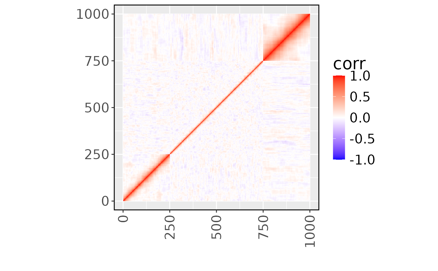
Only SNP 10 and SNP 950 have eQTL effects for all three cell types and for the first two cell types, respectively.
print(which(B != 0, arr.ind = TRUE))
#>      row col
#> [1,]  10   1
#> [2,] 950   1
#> [3,]  10   2
#> [4,] 950   2
#> [5,]  10   3
idx1 = 10
idx2 = 950
B[c(idx1, idx2), ]
#>           [,1]      [,2]      [,3]
#> [1,] 0.5477226 0.4472136 0.3162278
#> [2,] 0.5000000 0.3872983 0.0000000
Check the Z scores for the causal SNPs.
Z = matrix(0, M, C)
for (i in 1:M){
  m1 = summary(lm(Y ~ X[, i]))
  Z[i, ] = sapply(m1, function(x) x$coefficients[2, 3])
}
Z[c(idx1, idx2), ]
#>          [,1]     [,2]       [,3]
#> [1,] 5.162539 5.451293  3.7760017
#> [2,] 4.292018 3.878442 -0.1058495
Visualization of the Z scores for three cell types. The true eQTLs were surrounded with green circles. The dashed grey and red lines are for nominal significance () and significance after Bonferroni adjustment ().
df <- as.data.frame(Z)
colnames(df) = paste0("Cell_type_", 1:3)
df$SNP <- 1:nrow(df)

df_long <- pivot_longer(df,
                        cols = starts_with("Cell_type"),
                        names_to = "Variable",
                        values_to = "Z")
df_long$Highlight <- with(df_long,
  (SNP == 10) |
  (SNP == 950 & Variable != "Cell_type_3")
)

ggplot(df_long, aes(x = SNP, y = Z)) +
  geom_point() +
  geom_point(data = subset(df_long, Highlight),
             aes(x = SNP, y = Z),
             color = "green", size = 4, shape = 1) +
  geom_hline(yintercept = c(1.96, -1.96), linetype = "dashed", color = "grey") +
  geom_hline(yintercept = c(4.055, -4.055), linetype = "dashed", color = "red") +
  facet_wrap(~ Variable) +
  theme_minimal()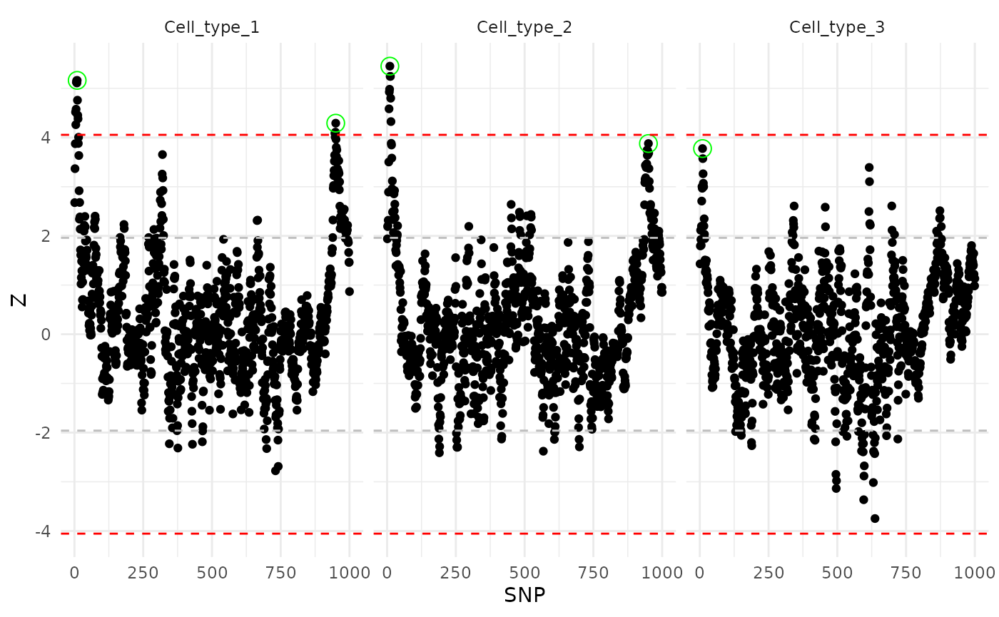
Fine-mapping
First, we try CASE fine-mapping for each cell type separately. The results lack power for the third cell type and for SNP 950.
for (c in 1:C){
  f1 = CASE(Z = Z[, c], R = R, N = N)
  print(f1$sets)
}
#> Start Prior fitting.
#> Initialize with patterns:  1 0
#> Start Posterior Analysis.
#> Start getting credible sets.
#> [[1]]
#> [[1]]$cs
#> [[1]]$cs[[1]]
#> [1]  7 10  8  9 11
#>
#>
#> [[1]]$purity_min_cor
#> [1] 0.8501335
#>
#> [[1]]$coverage
#> [1] 0.9716749
#>
#>
#> Start Prior fitting.
#> Initialize with patterns:  1 0
#> Start Posterior Analysis.
#> Start getting credible sets.
#> [[1]]
#> [[1]]$cs
#> [[1]]$cs[[1]]
#> [1] 10 11 12  9
#>
#>
#> [[1]]$purity_min_cor
#> [1] 0.8539356
#>
#> [[1]]$coverage
#> [1] 0.9519704
#>
#>
#> Start Prior fitting.
#> Initialize with patterns:  1 0
#> Start Posterior Analysis.
#> Start getting credible sets.
#> [[1]]
#> [[1]]$cs
#> list()
#>
#> [[1]]$purity_min_cor
#> numeric(0)
#>
#> [[1]]$coverage
#> numeric(0)
However, CASE jointly studies three cell types together to improve the power of identifying the causal variants.
fit <- CASE(Z = Z, R = R, N = N)
#> Start Prior fitting.
#> Initialize with patterns:  100 110 111 010 001 000
#> Start Posterior Analysis.
#> Start getting credible sets.
print(fit$sets)
#> [[1]]
#> [[1]]$cs
#> [[1]]$cs[[1]]
#> [1] 10 11
#>
#> [[1]]$cs[[2]]
#> [1] 950 947 949 951 948 952
#>
#>
#> [[1]]$purity_min_cor
#> [1] 0.9681014 0.9223080
#>
#> [[1]]$coverage
#> [1] 0.9655172 0.9593596
#>
#>
#> [[2]]
#> [[2]]$cs
#> [[2]]$cs[[1]]
#> [1] 10 11
#>
#> [[2]]$cs[[2]]
#> [1] 950 947 949 951 948 952
#>
#>
#> [[2]]$purity_min_cor
#> [1] 0.9681014 0.9223080
#>
#> [[2]]$coverage
#> [1] 0.9655172 0.9593596
#>
#>
#> [[3]]
#> [[3]]$cs
#> [[3]]$cs[[1]]
#> [1] 10 11
#>
#>
#> [[3]]$purity_min_cor
#> [1] 0.9681014
#>
#> [[3]]$coverage
#> [1] 0.96367
Session Information
sessionInfo()
#> R version 4.6.1 (2026-06-24)
#> Platform: x86_64-pc-linux-gnu
#> Running under: Ubuntu 24.04.4 LTS
#>
#> Matrix products: default
#> BLAS:   /usr/lib/x86_64-linux-gnu/openblas-pthread/libblas.so.3
#> LAPACK: /usr/lib/x86_64-linux-gnu/openblas-pthread/libopenblasp-r0.3.26.so;  LAPACK version 3.12.0
#>
#> locale:
#>  [1] LC_CTYPE=C.UTF-8       LC_NUMERIC=C           LC_TIME=C.UTF-8
#>  [4] LC_COLLATE=C.UTF-8     LC_MONETARY=C.UTF-8    LC_MESSAGES=C.UTF-8
#>  [7] LC_PAPER=C.UTF-8       LC_NAME=C              LC_ADDRESS=C
#> [10] LC_TELEPHONE=C         LC_MEASUREMENT=C.UTF-8 LC_IDENTIFICATION=C
#>
#> time zone: UTC
#> tzcode source: system (glibc)
#>
#> attached base packages:
#> [1] stats     graphics  grDevices utils     datasets  methods   base
#>
#> other attached packages:
#> [1] tidyr_1.3.2   ggplot2_4.0.3 CASE_0.3.1
#>
#> loaded via a namespace (and not attached):
#>  [1] gtable_0.3.6       jsonlite_2.0.0     dplyr_1.2.1        compiler_4.6.1
#>  [5] tidyselect_1.2.1   jquerylib_0.1.4    systemfonts_1.3.2  scales_1.4.0
#>  [9] textshaping_1.0.5  yaml_2.3.12        fastmap_1.2.0      R6_2.6.1
#> [13] labeling_0.4.3     generics_0.1.4     knitr_1.51         MASS_7.3-65
#> [17] tibble_3.3.1       desc_1.4.3         bslib_0.11.0       pillar_1.11.1
#> [21] RColorBrewer_1.1-3 rlang_1.2.0        cachem_1.1.0       xfun_0.59
#> [25] fs_2.1.0           sass_0.4.10        S7_0.2.2           otel_0.2.0
#> [29] cli_3.6.6          withr_3.0.3        pkgdown_2.2.0      magrittr_2.0.5
#> [33] digest_0.6.39      grid_4.6.1         mvtnorm_1.4-1      lifecycle_1.0.5
#> [37] vctrs_0.7.3        evaluate_1.0.5     glue_1.8.1         farver_2.1.2
#> [41] ragg_1.5.2         purrr_1.2.2        rmarkdown_2.31     tools_4.6.1
#> [45] pkgconfig_2.0.3    htmltools_0.5.9